
Thursday, 08 May 2021
autanabp
In the previous post we saw how to use Excel’s Vlookup function to unify data that is scattered in more than one listing as long as they had a single field in common.
Another situation where we can take advantage of this function is when we have two lists that a priori should coincide however they do not and we need to quickly identify which elements are missing from one list to another.
Let’s imagine that we have a master list of clients and on the other hand a list of clients that meet a certain condition. If what we want is to identify in a quick way that clients have not fulfilled this condition we can use the Vlookup function.
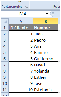
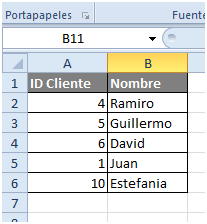
For the example we have a master list of customers in Sheet 1 of our book and in sheet 2 we have the customers who have already fulfilled the condition (whatever it is). In this example it is evident that clients of our master have not fulfilled the condition since with so few records it is easy, but there are times that we will have to know this among thousands of records. Let’s see how to do it.
In column C of our sheet1 we will enter the following formula:
=VLOOKUP(A2, Sheet2! A:B;2,0)
Creating this formula what we are doing is asking it to look for the value of A2 in column A (since it is the first of the matrix as we saw in the previous entry) and to return column number 2 of the search matrix (in this case having selected as range A: B what will return us will be the value of column B).
The result after dragging the formula on the rest of the rows is as follows:
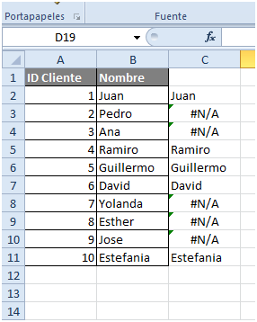
This means that at a quick glance we can tell which customers are on sheet1 but not on sheet2. They are all those that in column C have value #N/A, because that means that you have tried to look for our customer ID on sheet two and have not found it and therefore it is not there.
